Matching pCO₂ at Scale: Two Strategies for Robust Scale-Down Models
September 29, 2026
A scale-down model is only as useful as it is faithful. Bench-scale bioreactors are relied on across a product’s entire lifecycle: to evaluate process changes and de-risk technology transfer during development, and, once a process is running at scale, to troubleshoot deviations and test optimizations for commercial manufacturing without tying up production capacity. In every case, the value of the model depends on the same thing. If cells at the bench experience a different environment than they do at production scale, the conclusions don’t transfer.
Most scale-dependent parameters are straightforward to match: set power input per volume or sparge rate, and the automation does the rest. Dissolved CO₂ is an exception. It can’t be dialed in with a setpoint, because it results from gas transfer, bicarbonate chemistry, cell metabolism, and pH control all acting at once. Because bench vessels remove CO₂ far more efficiently than production vessels, the default outcome is a scale-down model that runs at lower pCO₂ than the process it is meant to represent.
The good news is that pCO₂ can be matched reliably with the right approach: treat it as a profile to match rather than a setpoint, choose the right lever for the size of the gap, and design the schedule with a model that captures how CO₂, pH, and metabolism feed back on each other. In this piece, we cover:
Why pCO₂ diverges between scales, and why that matters for your data
How to define the production-scale pCO₂ profile you are aiming for, whether or not at-scale data already exists
Two strategies for matching it at the bench, scheduled headspace overlay and CO₂ clamping, and when to use each
How Ark’s platform designs and tests these strategies in silico before you commit bench runs
The problem: pCO₂ doesn’t scale
Why production vessels accumulate more CO₂
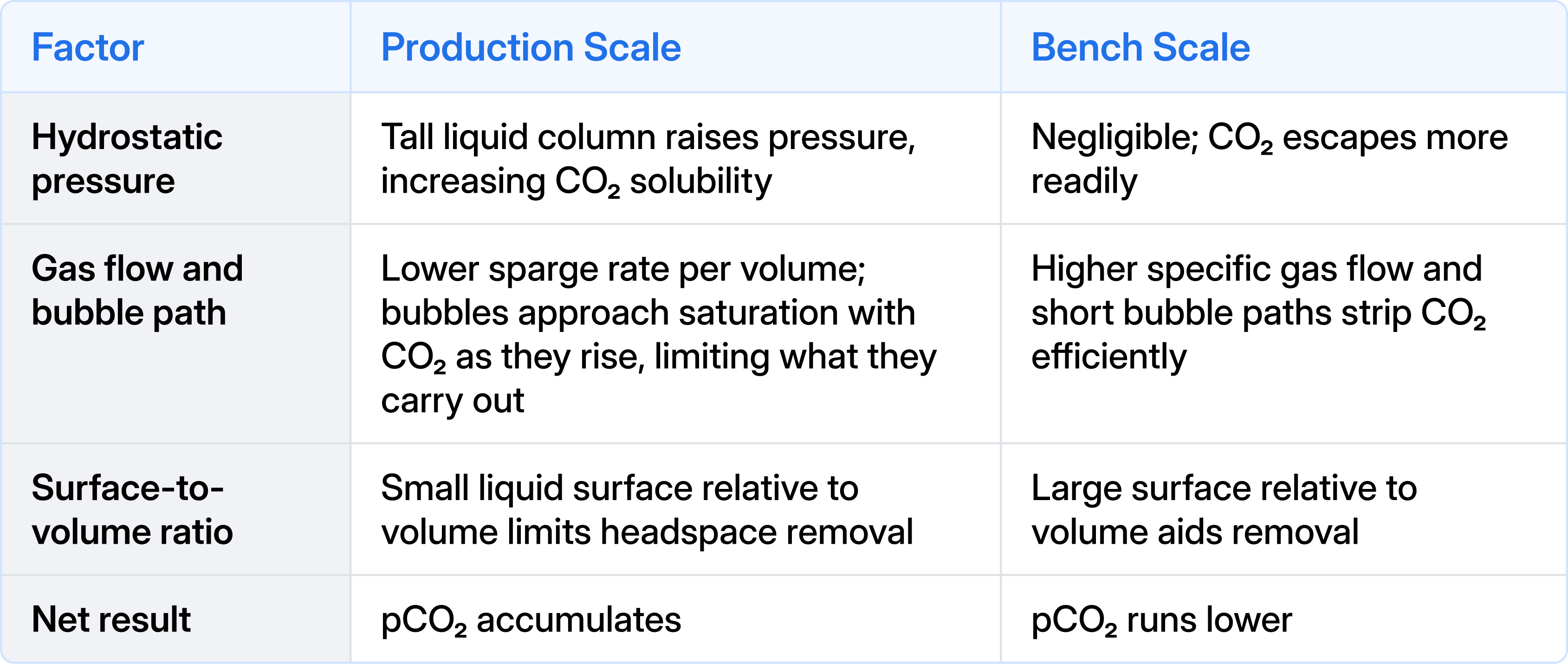
Cells produce CO₂ at roughly the same specific rate regardless of vessel size. What changes with scale is how efficiently that CO₂ is removed. Three physical differences work against large vessels: increased CO2 solubility, longer gas residence times, and surface-to-volume ratio. The effects of these differences are summarized in the table below.
Why it matters
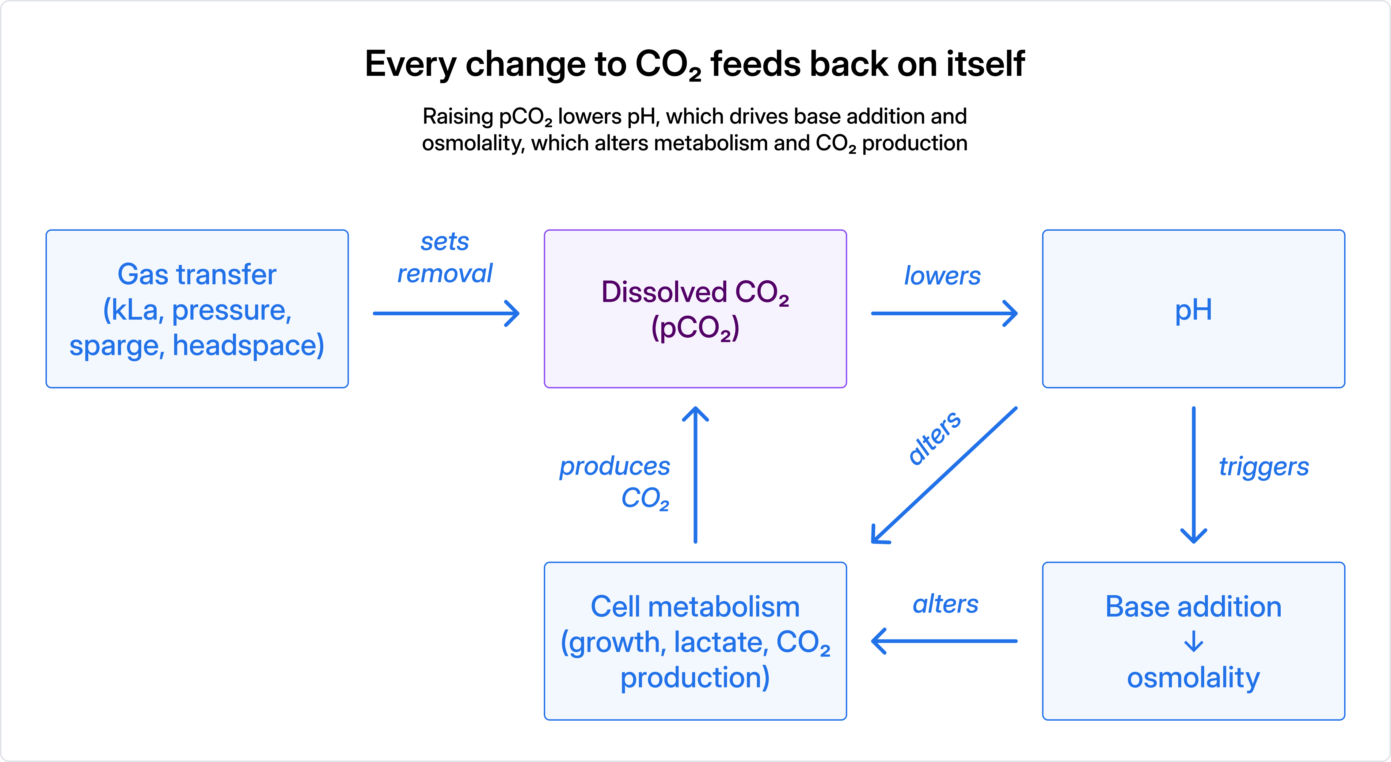
CO₂ is not a passive bystander. Dissolved CO₂ forms carbonic acid and lowers pH. The pH controller responds by adding base, which raises osmolality. Elevated pCO₂ and osmolality both affect cell growth, lactate metabolism, and product quality, and those changes in turn alter how much CO₂ the cells produce. The result is a feedback loop: change one variable and the others move with it.
Figure 1. The CO₂–pH–metabolism feedback loop
A bench model running at lower pCO₂ therefore isn’t just “off” on one number. It can use less base, run at lower osmolality, and show different growth and lactate behavior than production. That undermines the very comparisons it exists to support: a process change that looks neutral at the bench may not be at scale, and a deviation investigated at the bench may not reproduce at all. Unless CO₂ is deliberately matched, these discrepancies tend to show up as unexplained differences in growth, lactate, or product quality between scales, which are costly to diagnose after the fact.
The solution: match the profile in three steps
Matching pCO₂ comes down to three questions: What profile am I aiming for? Which lever should I use to hit it? And what side effects does that lever introduce? We take them in turn.
Step 1: Define the target profile
You can’t match what you haven’t defined, and the target is changing in time over the course of a run. Its level and shape determine which strategy you will need. Production-scale pCO₂ rises and falls with viable cell density and with pH control over the run. There are two ways to establish it:
From existing production data. For processes already running at scale, such as when troubleshooting a commercial deviation or optimizing an established process, use measured pCO₂ (online probes or offline blood-gas samples) alongside viable cell density, pH, and base addition from historical batches.
By prediction. For a new process or facility, there is no large-scale data yet, so the profile has to be predicted. At its core this is a balance: CO₂ produced (cellular metabolism plus bicarbonate conversion into CO2) versus CO₂ removed (the production vessel’s CO₂ mass-transfer coefficient, kLa, acting on the driving force set by pressure and gas flows). With a CO₂ kLa for the production vessel and CO₂ production rates from bench runs, a model can predict the full time course.
Getting the CO₂ kLa right: kLa is almost always characterized for oxygen, not CO₂. The two gases have different bulk volumetric gas transfer coefficients. One way to use an existing O2 kLa relationship for CO2 is to introduce a scalar value to adjust the O2 kLa. Theory based on relative diffusivities gives a starting value somewhat below one, but the effective ratio in a real vessel can differ, particularly at large scale where rising bubbles approach saturation with CO₂. Because CO₂ removal feeds directly into every prediction that follows, an inaccurate scalar biases both the target profile and the predicted effect of any overlay or clamping schedule. Where measured pCO₂ is available, the scalar should be calibrated against it rather than assumed.
Step 2: Choose a strategy
There are two main levers for raising bench-scale pCO2 to match a target pCO2 profile. They differ mainly in how much control they give you and how much they perturb the existing process.
Strategy 1: Scheduled headspace overlay
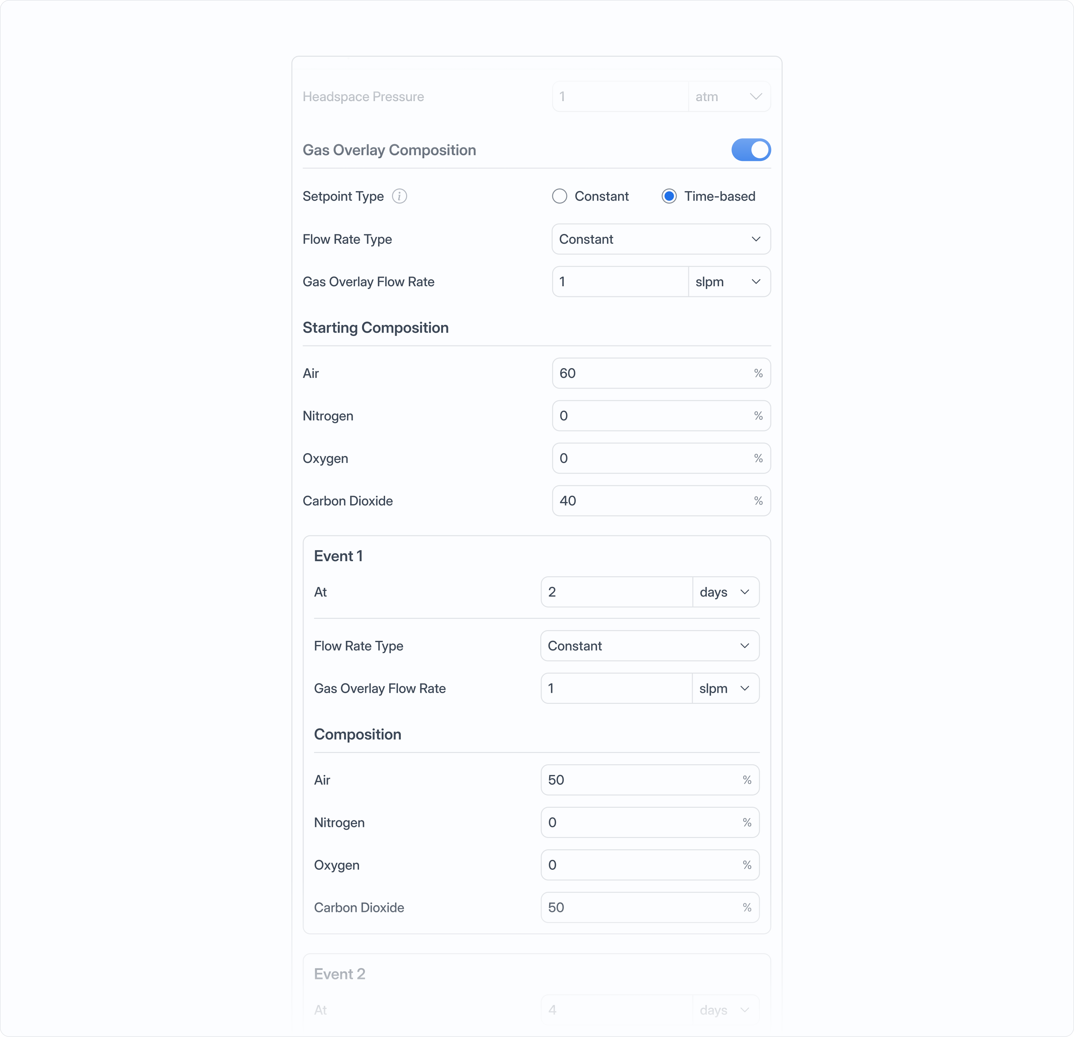
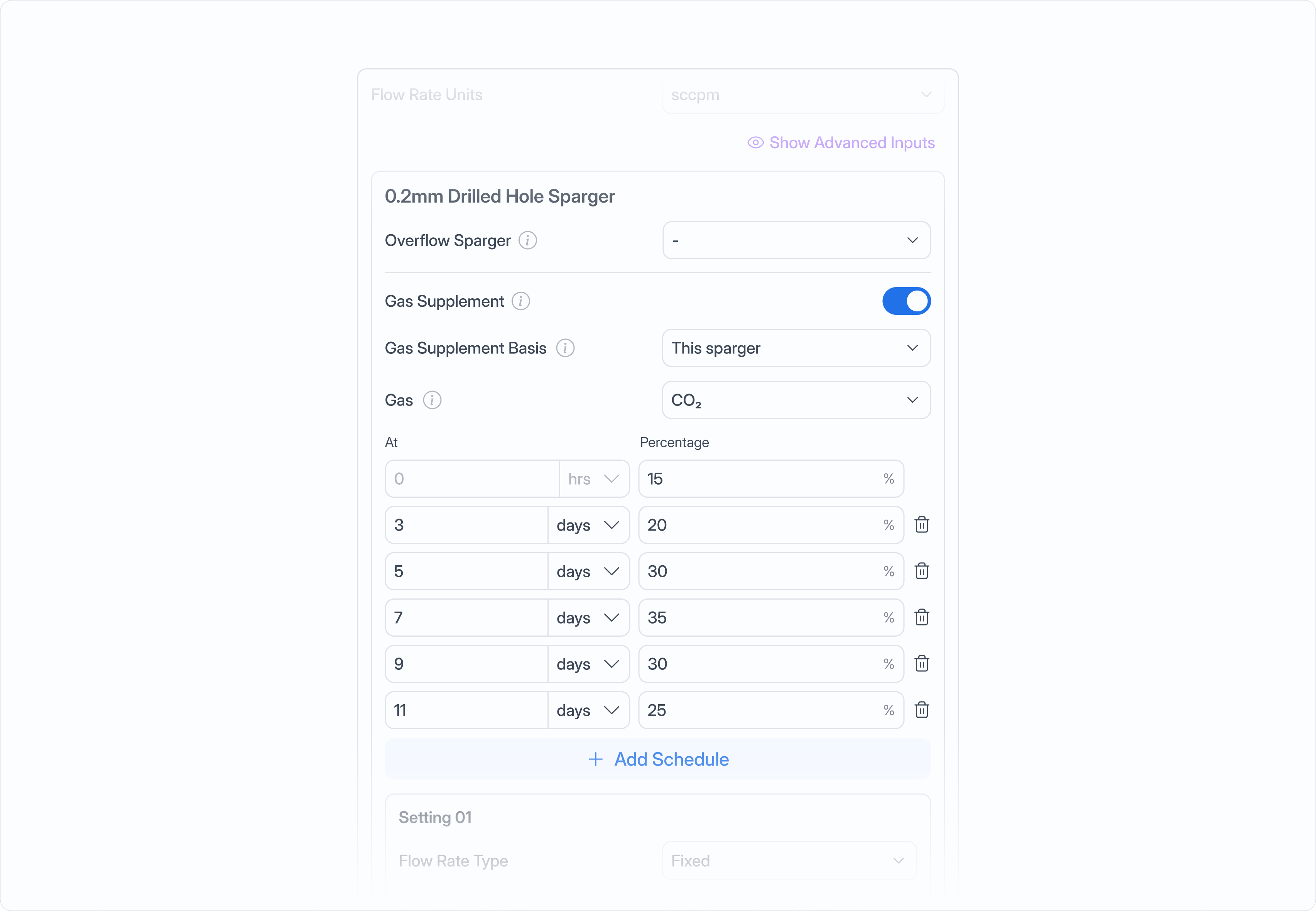
Figure 2. Gas overlay setup in the Ark app
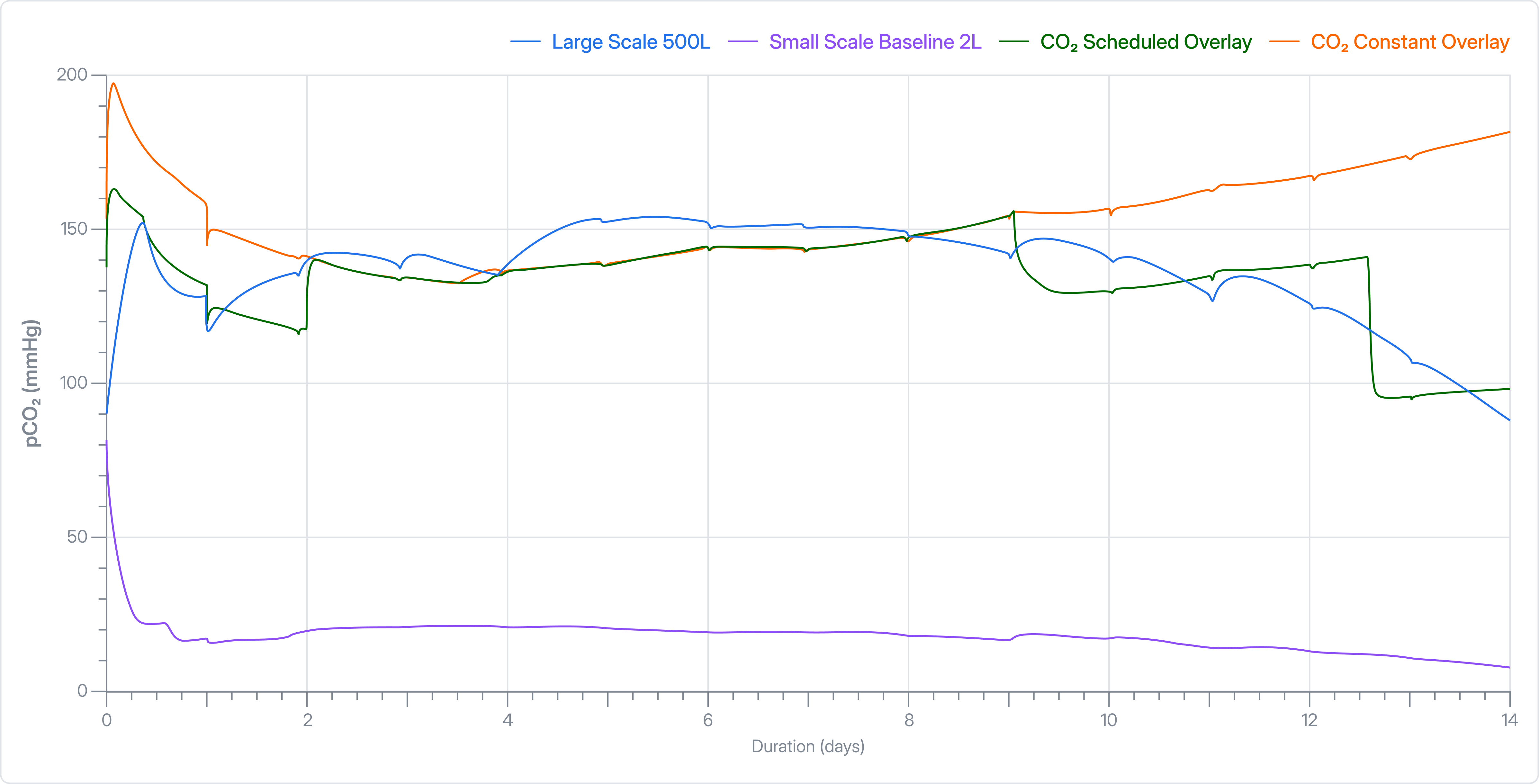
Figure 3. pCO2 profiles comparing an at-scale (500L process, blue) to the same process translated to the small scale (2L, purple). The pCO2 profiles differ greatly until a CO2 overlay is introduced. We show that a constant overlay (orange) captures the shift to higher pCO2 values at large scale but misses the details of the curvature. A scheduled overlay (green) does a good job of reproducing the large scale pCO2 profile.
How it works: CO₂ is added to the gas flowing over the liquid surface, reducing how much CO₂ escapes through the headspace and passively transferring CO2 into the liquid phase through the headspace.
Why use it: It is the least disruptive option. It works independently of the dissolved oxygen control and interacts weakly with pH control, so established control loops stay as they are.
What to watch: A constant overlay percentage is rarely enough. It raises the overall level of the profile but not its shape, so pCO₂ ends up too high early in the run and too low at peak. A scheduled overlay, where the CO₂ percentage steps up or down at defined points in the run, tracks the production profile far more closely (Figure 3). Because transfer through the liquid surface is limited, overlay also has less authority when the gap between scales is large.
Strategy 2: CO₂ clamping
Figure 4. CO2 clamping setup in the Ark app
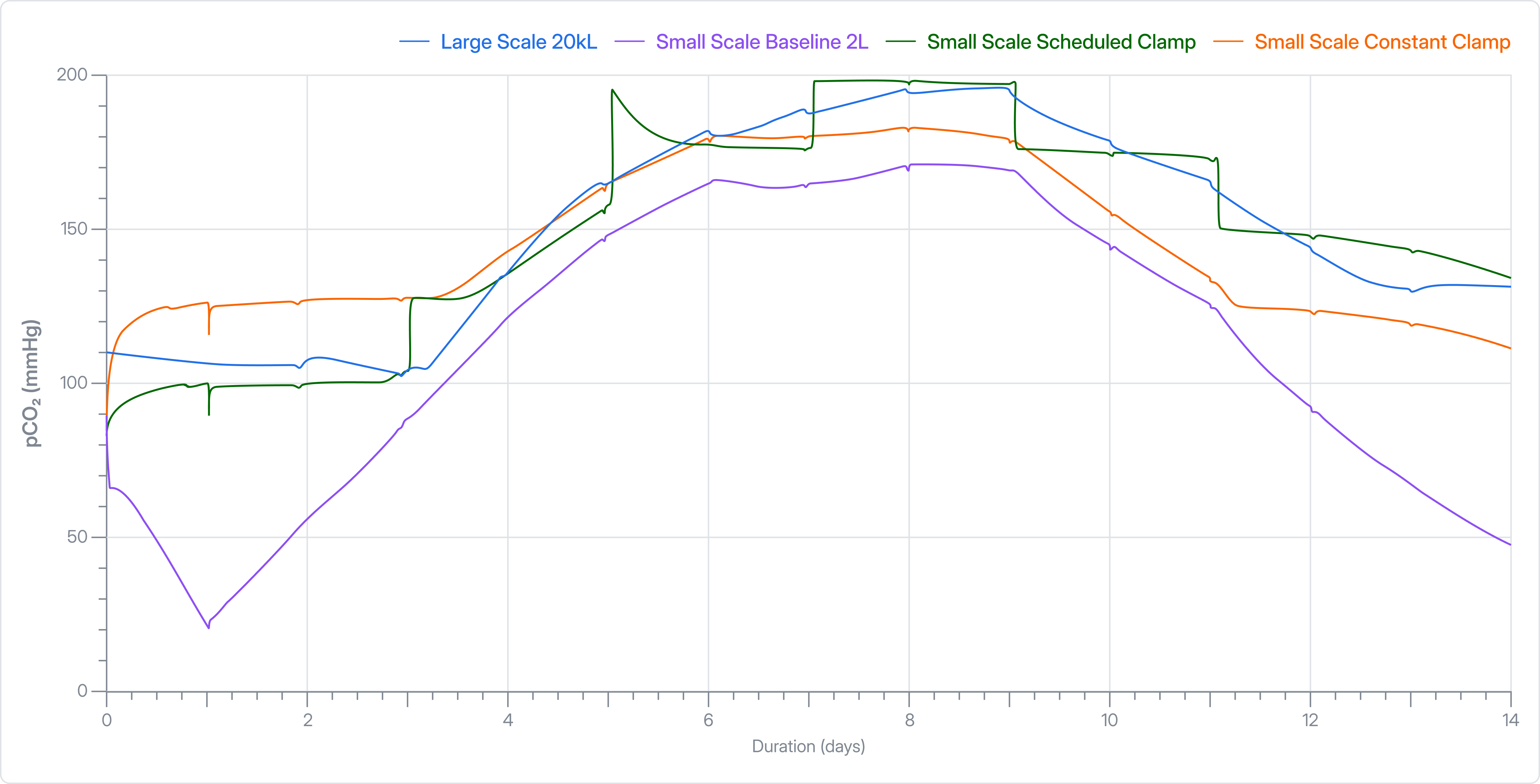
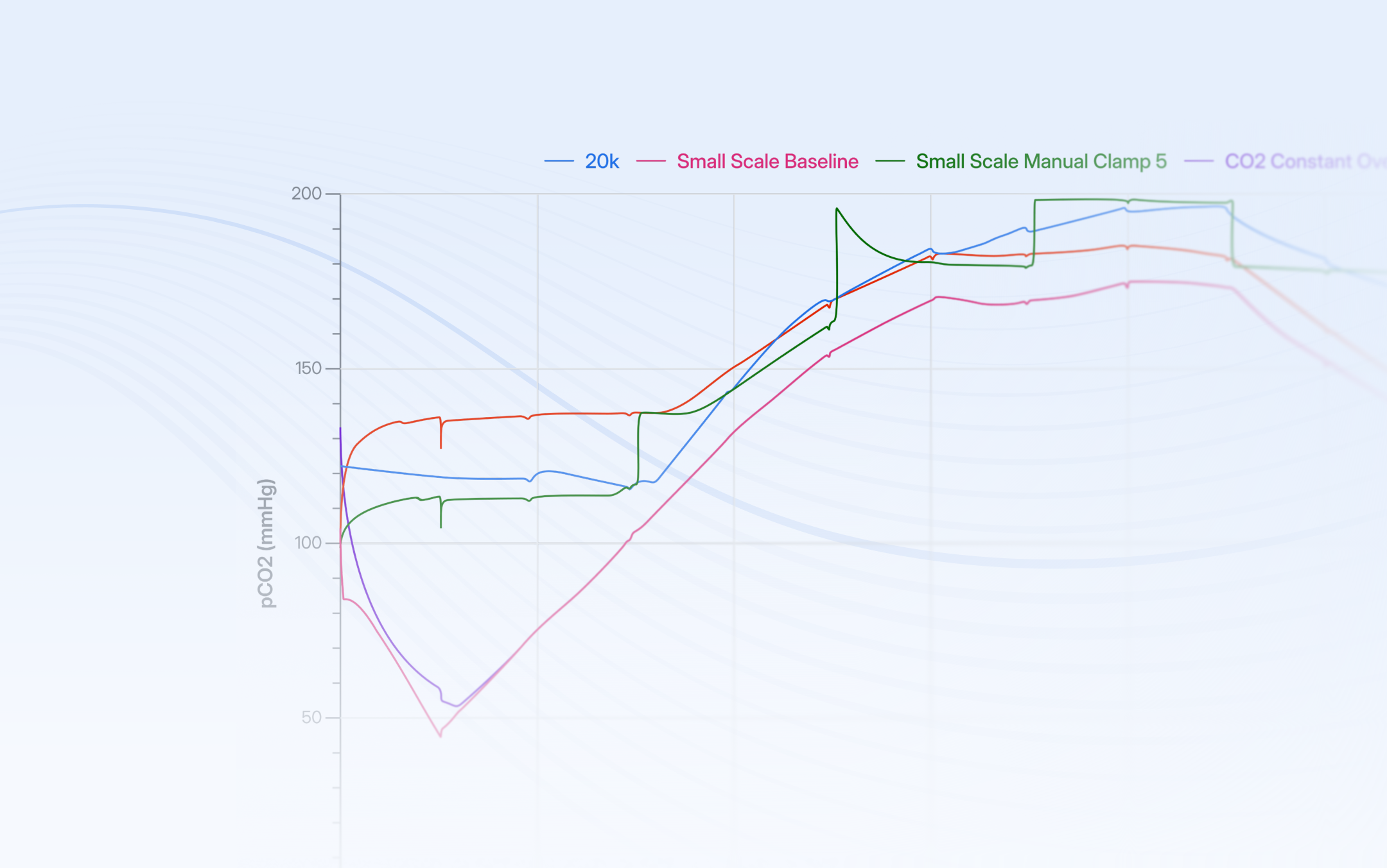
Figure 5. Illustrative pCO₂ profiles. A scale down model from a 20kL reactor (blue) to a 2L reactor (baseline process in purple). Adding an aggressive CO2 overlay (not shown) is insufficient here because the pCO2 is driven primarily by high-side pH control. Using CO2 clamping, we obtain a better agreement using a constant (orange) and scheduled (green) strategy.
How it works: CO₂ is added to the sparge gas at a fixed or scheduled fraction of the total sparge flow. Because the gas bubbling through the liquid now carries CO₂, dissolved CO₂ is driven toward a target equilibrium.
Why use it: It is the stronger lever. Clamping acts directly on the bulk liquid, so it can hold the target precisely even when bench and production differ substantially. Clamping scale-down models are also less sensitive to kLa as the additional CO2 in the sparged gases drives pCO2 towards thermodynamic equilibrium.
What to watch: It changes more of the process. Adding CO₂ to the sparge increases total gas flow, which can alter oxygen transfer and how the DO controller responds. Higher pCO₂ also lowers pH, increasing base addition and osmolality, and may influence cell metabolism directly. These effects need to be characterized before clamping is relied on (see Step 3).
Side by side
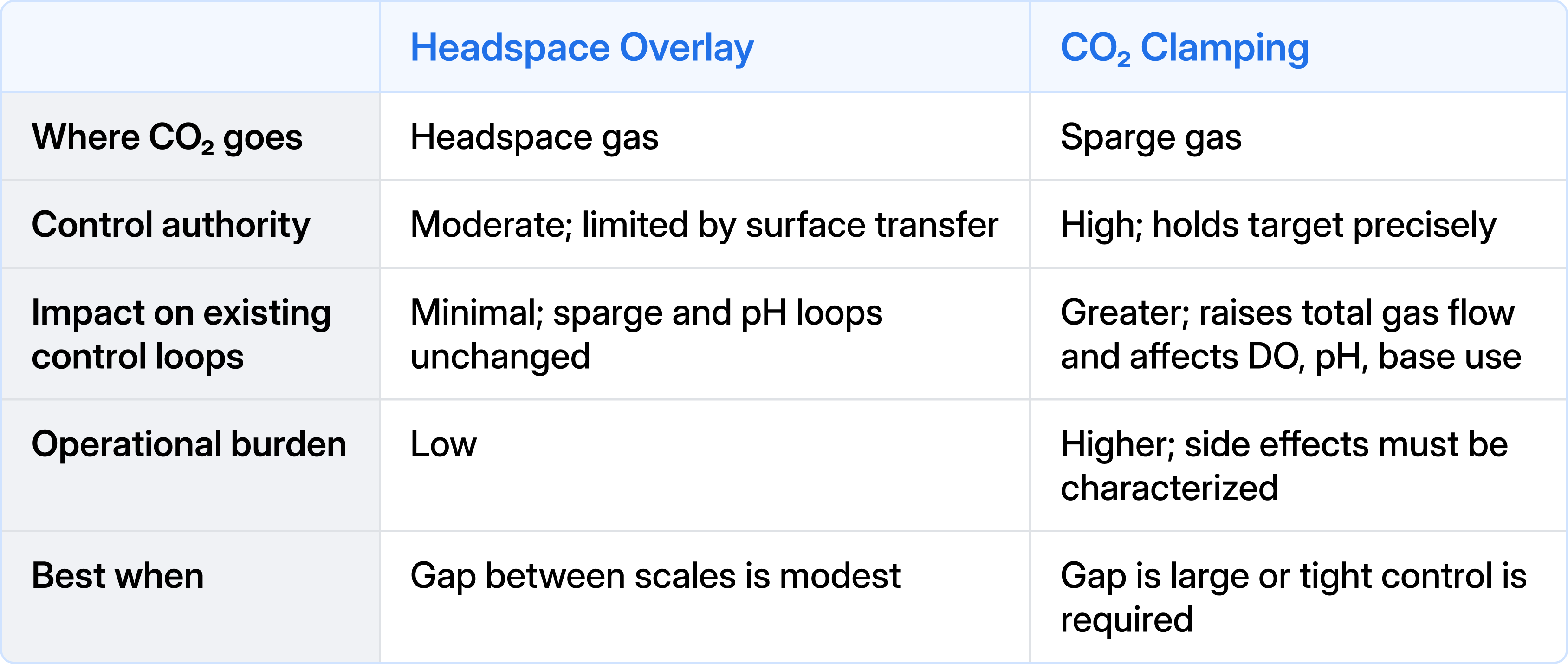
Choosing the right strategy depends on the specifics of your scale down problem, but if there is enough confidence in kLa, metabolic CO2 production rates are known, and the difference between scales is not major, headspace overlay is a good place to start. When there is uncertainty in these parameters, when the scale difference is large, or when the application demands tight control, clamping is usually the preferred option.
Step 3: Characterize side effects and verify
Matching pCO₂ is not the finish line. Whichever strategy you choose, confirm that pH, osmolality, and metabolism track production too, and that the strategy hasn’t introduced new differences of its own. This matters most for clamping. A practical approach:
Simulate first. Predict how the schedule will change pH, base flow rates, sparge rates, and other process parameters before running anything.
Run a small confirmation set. Run the schedule at bench scale alongside a control. Track pCO₂ (offline blood gas), pH, cumulative base addition, osmolality, DO controller output, viable cell density, lactate, titer, and key quality attributes.
Compare and adjust. Check the measured pCO₂ against the target profile and confirm that base use, osmolality, and metabolism move the way production does. Refine the schedule where they don’t.
In practice, this is often less burdensome than it sounds. In the real cell culture datasets we have worked with, both of these strategies have not resulted in dramatic metabolic behavioral changes at the small scale.
How Ark’s platform can be used to accurately match pCO2
The hard part of CO₂ matching is the feedback loop shown in Figure 1. Every adjustment you make to raise pCO₂ ripples through pH, base addition, osmolality, and metabolism, and those changes feed back on CO₂ itself. A static calculation misses these interactions, and empirical tuning only discovers them one bench run at a time.
Ark’s platform simulates the loop as a whole. Gas transfer and carbonate chemistry are governed by mechanistic, physics-based models, with machine learning capturing cell behavior within a set of rigorous biological constraints. Because the scale-dependent differences are physical, this grounding lets the platform predict conditions that have never been run, rather than being limited to the operating strategies in its training data. It learns more from less data and extrapolates with confidence.
In practice, the workflow looks like this:
Define the target. Use historical production data where it exists, or predict the production-scale pCO₂ profile from kLa estimates, a CO₂ scalar calibrated against measured pCO₂, and cellular CO₂ production rates.
Design the schedule. Derive overlay or clamping schedules and optimize them directly in the Ark platform to minimize deviation from the target profile.
Stress-test it. Run sensitivity analyses to see how robust each schedule is to uncertainty in kLa, the CO₂ scalar, CO₂ production rates, and other key inputs.
Predict the knock-on effects. Forecast the impact on pH, base addition, lactate, critical quality attributes, and titer, so teams can evaluate the altered conditions they are likely to see at production scale.
Confirm at the bench. Run a small number of verification experiments instead of an extended tuning campaign.
Because the approach requires minimal small-scale experimental data, teams can arrive at a CO₂ strategy with far fewer bench runs than empirical tuning, and apply the same workflow whether they are developing a new process, transferring it, or troubleshooting and optimizing one already in commercial production.
Key takeaways
Dissolved CO₂ is too dynamic to match with a static process change. Treat it as a time-course profile.
Bench-scale pCO₂ runs lower as compared to larger scales. This difference propagates to pH, osmolality, metabolism, and other process parameters.
Define the production-scale target first, from historical data or by prediction, using a CO₂ scalar for kLa calibrated to measured pCO₂.
Use a scheduled headspace overlay when the gap is modest and when there is high confidence in bioreactor characterization; use CO₂ clamping when the gap is large or control must be tight, after characterizing its side effects.
A model that captures the CO₂–pH–metabolism feedback loop lets you design and stress-test schedules in silico, dramatically reducing iteration cycles and providing more insights into the tight coupling of bioprocess time-series data.
Written by Nick Austin, Head of Modeling
Thanks to Jongchan Lee, Alex Williams, Natoiwoki Mollel, and Ping Xu of Bristol Myers Squibb for pointing us to the clamping strategy work.